Threshold-free cluster enhancement (TFCE) in CoSMoMVPA

It is assumed here that the reader is already somewhat familiar with the TFCE procedure and can use CoSMoMVPA.

While the 2016 Frontiers paper introduces the framework of CoSMoMVPA, the exact details of how it implements threshold-free cluster enhancement (TFCE) for multiple-comparisons correction are somewhat opaque. This blog post is aimed at describing those details.

The principle

As I understand it, using TFCE we perform voxel-level inference about the existence of an effect while accounting for the “support” of neighbouring voxels towards the existence of that effect at the given voxel. If the given voxel is a part of a “hill” on a variable’s landscape, both the extent of that hill and the value of the variable at the given voxel contribute towards the inference about that value being higher than baseline.

There are two steps in this procedure:

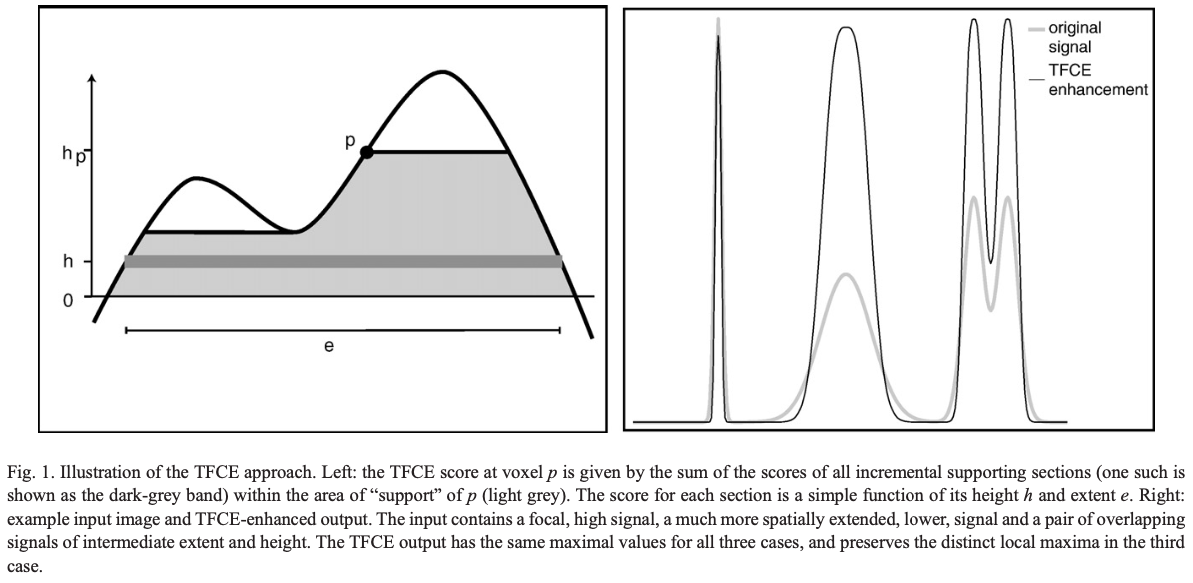
1. Computing a new variable, the TFCE value, which quantifies the amount of “support” a voxel has - exemplified in the image below (Fig 1. from the TFCE paper).
2. Computing the null distribution of TFCE values at every voxel, then computing z-scores on these distributions for the values computed in step 1, which can then be thresholded for each voxel at a desired false discovery rate for statistical inference.

Computing the TFCE value

E and H are constants which weigh the contribution of the cluster extent (e) and height (h) towards the TFCE value. While the above formula defines TFCE, in CoSMoMVPA it is computed in an iterative procedure as follows.

Let’s say the maximum value of the relevant variable (e.g. GLM weights in fMRI) across voxels is \(h_m\). Then we define \(\approx (h_m-h_0)/\Delta h\) markers between \(h_0\) and \(h_m\), where \(h_0\) is the baseline value (e.g. 0 in the case of fMRI GLM weights, or 50 in the case of binary classification accuracy. Note that these raw scores are not directly used to compute the TFCE values, as explained later). At every marker, we list the voxels with values above the value of the marker. We then identify the largest possible clusters with contiguous voxels. In each cluster, every voxel’s TFCE value is incremented by \(\Delta h(\text{# of voxels in the cluster})^E(\text{value of the marker})^H\), where usually \(\Delta h = 0.1\), \(E = 0.5\), and \(H = 2\) (check out the TFCE paper for justification).

This computation of TFCE values is done with the function cosmo_measure_clusters in CoSMoMVPA.

This procedure is repeated after flipping the variable values around the baseline value, to quantify the TFCE values for any voxels with values below the baseline. Two sets of TFCE values are returned (each voxel is positive either in one or none of the maps) which are then compared against the null distribution as explained in the next section.

In a typical neuroimaging analysis, we have values for a given variable across voxels of the aligned brains of N participants (e.g. in MNI space). The TFCE values are computed across the voxels over a measure of the standardized mean across participants. Precisely, for each voxel, after subtracting the baseline value, the mean across participants is divided by the standard error, which is then transformed with the Student’s-T cumulative distribution function (CDF), which is finally transformed to a z-score with the inverse normal CDF. This is the variable over which TFCE values are calculated.

The null distribution and statistical inference

As we are usually interested in inferring if a voxel’s value is above/below baseline, we would want to compare that value to a null distribution of values that are equally spread around the baseline. In CoSMoMVPA, this is accomplished by iteratively flipping the sign of the voxel values of a random half of the participants (after subtracting the baseline value). This ensures that the expected mean across iterations, for each voxel, is equal to the baseline. For each iteration, the TFCE values are computed, separately for the positively and negatively valued voxels, as above, to generate null distributions of TFCE values for both the positively and negatively valued voxels respectively.

In the case of a positively valued voxel, the iterations where the z-scores (obtained after the standardization procedure explained earlier) are positive for that voxel, are considered. The number of iterations where the TFCE values are less than the actual TFCE value of that voxel is computed. If that number is more than half of the total number of iterations, that number is scaled to lie between 0.5 and 1 (1 where all iterations yield lower TFCE values than the actual value). Similarly, for a negatively valued voxel, that number is scaled to lie between 0 (0 where all iterations yield lower TFCE values than the actual one) and 0.5. Then using the inverse normal CDF, a z-score is computed for each voxel which is the output of the entire procedure.

For statistical inference, if we wish to restrict the false discovery rate to, say, 5%, we can threshold the final output at \(z\geq1.96\) and \(z\leq-1.96\).

Example script

Adapted from CoSMoMVPA demo code.

% Let ds.samples contains the voxel values (e.g. output of a searchlight analysis) across the aligned brains of N participants.

% Compute voxel neighborhoods (used in the clustering procedure required during TFCE computation)
cluster_nbrhood = cosmo_cluster_neighborhood(ds);

% Parameters of the procedure
opt = struct();
opt.niter = 10000; % generate the null distribution with 10000 iterations
opt.h0_mean = 0; % baseline value
opt.null = [];

% Compute the TFCE values (cosmo_measure_clusters is called within this function) and output the z-scores
tfce_zscores = cosmo_montecarlo_cluster_stat(ds,cluster_nbrhood,opt);

% Compute z-threshold for statistical inference
p = 0.05;
z_th = norminv(1-p/2); % two-sided test

% Create thresholded maps and save them
pos_voxs = tfce_zscores.samples >= z_th;
neg_voxs = tfce_zscores.samples <= -z_th;

% map of all responses significantly above the baseline
tfce_zscores.samples = pos_voxs;
cosmo_map2fmri(tfce_zscores, 'pos_voxs.nii'); 

% map of all responses significantly below the baseline
tfce_zscores.samples = neg_voxs;
cosmo_map2fmri(tfce_zscores, 'neg_voxs.nii');